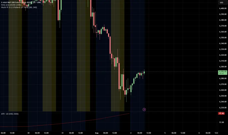
3-1-3 PatternThis Pine Script indicator analyzes and visualizes a specific candlestick pattern called the "3-1-3 Pattern" across multiple timeframes. Here's what it does:
Core Functionality
Pattern Detection: The script looks for a 7-bar candlestick pattern:
Bearish 3-1-3: 3 red candles + 1 green candle + 3 red candles
Bullish 3-1-3: 3 green candles + 1 red candle + 3 green candles
Visual Output
When a 3-1-3 pattern is detected, the script:
Creates a colored box around the middle bar (bar 3) of the pattern
Adds a small label showing the pattern type ("Bear 1H" or "Bull 4H", etc.)
Extends the box forward until the price breaks above the pattern's high or below its low
Pattern Management
The script actively manages the patterns by:
Tracking active patterns for each timeframe separately
Removing expired patterns when price breaks the pattern's high/low levels
Extending boxes to the current time to keep them visible
Practical Use
This indicator helps traders:
Spot reversal patterns across multiple timeframes simultaneously
See confluence when patterns align on different timeframes
Track pattern validity (boxes disappear when invalidated by price action)
Essentially, it's a multi-timeframe pattern recognition tool that automatically identifies and tracks these specific 7-bar reversal patterns on your chart.
Cari dalam skrip untuk "THE SCRIPT"
Ultimate JLines & MTF EMA (Configurable, Labels)## Ultimate JLines & MTF EMA (Configurable, Labels) — Script Overview
This Pine Script is a comprehensive, multi-timeframe indicator based on J Trader concepts. It overlays various Exponential Moving Averages (EMAs), VWAP, inside bar highlights, and dynamic labels onto price charts. The script is highly configurable, allowing users to tailor which elements are displayed and how they appear.
### Key Features
#### 1. **Multi-Timeframe JLines**
- **JLines** are pairs of EMAs (default lengths: 72 and 89) calculated on several timeframes:
- 1 minute (1m)
- 3 minutes (3m)
- 5 minutes (5m)
- 1 hour (1h)
- Custom timeframe (user-selectable)
- Each pair can be visualized as individual lines and as a "cloud" (shaded area between the two EMAs).
- Colors and opacity for each timeframe are user-configurable.
#### 2. **200 EMA on Multiple Timeframes**
- Plots the 200-period EMA on selectable timeframes: 1m, 3m, 5m, 15m, and 1h.
- Each can be toggled independently and colored as desired.
#### 3. **9 EMA and VWAP**
- Plots a 9-period EMA, either on the chart’s current timeframe or a user-specified one.
- Plots VWAP (Volume-Weighted Average Price) for additional trend context.
#### 4. **5/15 EMA Cross Cloud (5min)**
- Calculates and optionally displays a shaded "cloud" between the 5-period and 15-period EMAs on the 5-minute chart.
- Highlights bullish (5 EMA above 15 EMA) and bearish (5 EMA below 15 EMA) conditions with different colors.
- Optionally displays the 5 and 15 EMA lines themselves.
#### 5. **Inside Bar Highlighting**
- Highlights bars where the current high is less than or equal to the previous high and the low is greater than or equal to the previous low (inside bars).
- Color is user-configurable.
#### 6. **9 EMA / VWAP Cross Arrows**
- Plots up/down arrows when the 9 EMA crosses above or below the VWAP.
- Arrow colors and visibility are configurable.
#### 7. **Dynamic Labels**
- On the most recent bar, displays labels for each enabled line (EMAs, VWAP), offset to the right for clarity.
- Labels include the timeframe, type, and current value.
### Customization Options
- **Visibility:** Each plot (line, cloud, arrow, label) can be individually toggled on/off.
- **Colors:** All lines, clouds, and arrows can be colored to user preference, including opacity for clouds.
- **Timeframes:** JLines and EMAs can be calculated on different timeframes, including a custom one.
- **Label Text:** Labels dynamically reflect current indicator values and are color-coded to match their lines.
### Technical Implementation Highlights
- **Helper Functions:** Functions abstract away the logic for multi-timeframe EMA calculation.
- **Security Calls:** Uses `request.security` to fetch data from other timeframes, ensuring accurate multi-timeframe plotting.
- **Efficient Label Management:** Deletes old labels and creates new ones only on the last bar to avoid clutter and maintain performance.
- **Conditional Plotting:** All visual elements are conditionally plotted based on user input, making the indicator highly flexible.
### Use Cases
- **Trend Identification:** Multiple EMAs and VWAP help traders quickly identify trend direction and strength across timeframes.
- **Support/Resistance:** 200 EMA and JLines often act as dynamic support/resistance levels.
- **Entry/Exit Signals:** Crosses between 9 EMA and VWAP, as well as 5/15 EMA clouds, can signal potential trade entries or exits.
- **Pattern Recognition:** Inside bar highlights aid in spotting consolidation and breakout patterns.
### Summary Table of Configurable Elements
| Feature | Timeframes | Cloud Option | Label Option | Color Customizable | Description |
|----------------------------|-------------------|--------------|--------------|--------------------|-----------------------------------------------|
| JLines (72/89 EMA) | 1m, 3m, 5m, 1h, Custom | Yes | Yes | Yes | Key trend-following EMAs with cloud fill |
| 200 EMA | 1m, 3m, 5m, 15m, 1h | No | Yes | Yes | Long-term trend indicator |
| 9 EMA | Any | No | Yes | Yes | Short-term trend indicator |
| VWAP | Chart TF | No | Yes | Yes | Volume-weighted average price |
| 5/15 EMA Cloud (5m) | 5m | Yes | No | Yes | Bullish/bearish cloud between 5/15 EMAs |
| Inside Bar Highlight | Chart TF | No | N/A | Yes | Highlights price consolidation |
| 9 EMA / VWAP Cross Arrows | Chart TF | No | N/A | Yes | Marks EMA/VWAP crossovers with arrows |
This script is ideal for traders seeking a robust, multi-timeframe overlay that combines trend, momentum, and pattern signals in a single, highly customizable indicator. I do not advocate to subscribe to JTrades or the system they tout. This is based on my own observations and not a copy of any JTrades scripts. It is open source to allow full transparency.

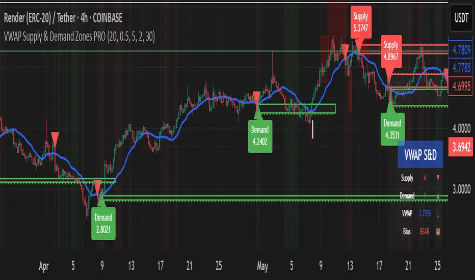
VWAP Supply & Demand Zones PRO**Overview:**
This script represents a major evolution of the original "VWAP Supply and Demand Zones" indicator. Initially created to explore price interaction with VWAP, it has now matured into a robust and feature-rich tool for identifying high-probability zones of institutional buying and selling pressure. The update introduces volume and momentum validation, dynamic zone management, alert logic, and a visual dashboard (HUD) — all designed for improved precision and clarity. The structural improvements, anti-repainting logic, and significant added utility warranted releasing this as a new script rather than a minor update.
---
### What It Does:
This indicator dynamically detects **supply and demand zones** using VWAP-based logic combined with **volume** and **momentum confirmation**. When price crosses VWAP with strength, it identifies the potential zone of excess demand (below VWAP) or supply (above VWAP), marking it visually with colored regions on the chart.
Each zone is extended for a user-defined duration, monitored for touch interactions (tests), and tracked for possible breaks. The script helps traders interpret price behavior around these institutional zones as either **reversal** opportunities or **continuation** confirmation depending on context and strategy preference.
---
### How It Works:
* **VWAP Basis**: Zones are anchored at VWAP at the time of a significant cross.
* **Volume & Momentum Filters**: Crosses are only considered valid if backed by above-average volume and notable price momentum.
* **Zone Drawing**: Validated supply and demand zones are drawn as boxes on the chart. Each is extended forward for a customizable number of bars.
* **Touch Counting**: Zones track the number of price touches. Alerts are issued after a user-defined number of tests.
* **Break Detection**: If price closes significantly beyond a zone boundary, the zone is marked as broken and visually dimmed.
* **Visual Dashboard (HUD)**: A compact real-time HUD displays VWAP value, active zone counts, and current market bias.
---
### How to Use It:
**Reversal Trading:**
* Look for price **rejecting** a zone after touching it.
* Use rejection candles or secondary indicators (e.g., RSI divergence) to confirm.
* These setups may offer low-risk entries when price respects the zone.
**Continuation Trading:**
* A **break of a zone** suggests strong directional bias.
* Use confirmed zone breaks to enter in the direction of momentum.
* Ideal in trending environments, especially with high volume and ATR movement.
---
### Key Inputs:
* **VWAP Length**: Moving VWAP period (default: 20)
* **Zone Width %**: Percentage size of zone buffer (default: 0.5%)
* **Min Touches**: How many times price must test a zone before alerts trigger
* **Zone Extension**: How far into the future zones are projected
* **Volume & ATR Filters**: Ensure only strong, valid crossovers create zones
---
### Alerts:
You can enable alerts for:
* **New zone creation**
* **Zone tests (after minimum touch count)**
* **Zone breaks**
* **VWAP crosses**
* **Active presence inside a zone (entry conditions)**
These alerts help automate market monitoring, making it suitable for discretionary or systematic workflows.
---
### Why It's a New Script:
This is not a cosmetic update. The internal logic, signal generation, filtering methodology, visual engine, and UX framework have been entirely rebuilt from the ground up. The result is a highly adaptive, precision-oriented tool — appropriate for intraday scalpers and swing traders alike. It goes far beyond the original in terms of functionality and reliability, justifying a fresh release.
---
### Suitable Markets and Timeframes:
* Works across all liquid markets (crypto, equities, futures, forex)
* Best used on timeframes where volume data is stable (5m and above recommended)
* Recalibrate inputs for optimal detection across instruments
FvgPanel█ OVERVIEW
This library provides functionalities for creating and managing a display panel within a Pine Script™ indicator. Its primary purpose is to offer a structured way to present Fair Value Gap (FVG) information, specifically the nearest bullish and bearish FVG levels across different timeframes (Current, MTF, HTF), directly on the chart. The library handles the table's structure, header initialization, and dynamic cell content updates.
█ CONCEPTS
The core of this library revolves around presenting summarized FVG data in a clear, tabular format. Key concepts include:
FVG Data Aggregation and Display
The panel is designed to show at-a-glance information about the closest active FVG mitigation levels. It doesn't calculate these FVGs itself but relies on the main script to provide this data. The panel is structured with columns for timeframes (TF), Bullish FVGs, and Bearish FVGs, and rows for "Current" (LTF), "MTF" (Medium Timeframe), and "HTF" (High Timeframe).
The `panelData` User-Defined Type (UDT)
To facilitate the transfer of information to be displayed, the library defines a UDT named `panelData`. This structure is central to the library's operation and is designed to hold all necessary values for populating the panel's data cells for each relevant FVG. Its fields include:
Price levels for the nearest bullish and bearish FVGs for LTF, MTF, and HTF (e.g., `nearestBullMitLvl`, `nearestMtfBearMitLvl`).
Boolean flags to indicate if these FVGs are classified as "Large Volume" (LV) (e.g., `isNearestBullLV`, `isNearestMtfBearLV`).
Color information for the background and text of each data cell, allowing for conditional styling based on the FVG's status or proximity (e.g., `ltfBullBgColor`, `mtfBearTextColor`).
The design of `panelData` allows the main script to prepare all display-related data and styling cues in one object, which is then passed to the `updatePanel` function for rendering. This separation of data preparation and display logic keeps the library focused on its presentation task.
Visual Cues and Formatting
Price Formatting: Price levels are formatted to match the instrument's minimum tick size using an internal `formatPrice` helper function, ensuring consistent and accurate display.
Large FVG Icon: If an FVG is marked as a "Large Volume" FVG in the `panelData` object, a user-specified icon (e.g., an emoji) is prepended to its price level in the panel, providing an immediate visual distinction.
Conditional Styling: The background and text colors for each FVG level displayed in the panel can be individually controlled via the `panelData` object, enabling the main script to implement custom styling rules (e.g., highlighting the overall nearest FVG across all timeframes).
Handling Missing Data: If no FVG data is available for a particular cell (i.e., the corresponding level in `panelData` is `na`), the panel displays "---" and uses a specified background color for "Not Available" cells.
█ CALCULATIONS AND USE
Using the `FvgPanel` typically involves a two-stage process: initialization and dynamic updates.
Step 1: Panel Creation
First, an instance of the panel table is created once, usually during the script's initial setup. This is done using the `createPanel` function.
Call `createPanel()` with parameters defining its position on the chart, border color, border width, header background color, header text color, and header text size.
This function initializes the table with three columns ("TF", "Bull FVG", "Bear FVG") and three data rows labeled "Current", "MTF", and "HTF", plus a header row.
Store the returned `table` object in a `var` variable to persist it across bars.
// Example:
var table infoPanel = na
if barstate.isfirst
infoPanel := panel.createPanel(
position.top_right,
color.gray,
1,
color.new(color.gray, 50),
color.white,
size.small
)
Step 2: Panel Updates
On each bar, or whenever the FVG data changes (typically on `barstate.islast` or `barstate.isrealtime` for efficiency), the panel's content needs to be refreshed. This is done using the `updatePanel` function.
Populate an instance of the `panelData` UDT with the latest FVG information. This includes setting the nearest bullish/bearish mitigation levels for LTF, MTF, and HTF, their LV status, and their desired background and text colors.
Call `updatePanel()`, passing the persistent `table` object (from Step 1), the populated `panelData` object, the icon string for LV FVGs, the default text color for FVG levels, the background color for "N/A" cells, and the general text size for the data cells.
The `updatePanel` function will then clear previous data and fill the table cells with the new values and styles provided in the `panelData` object.
// Example (inside a conditional block like 'if barstate.islast'):
var panelData fvgDisplayData = panelData.new()
// ... (logic to populate fvgDisplayData fields) ...
// fvgDisplayData.nearestBullMitLvl = ...
// fvgDisplayData.ltfBullBgColor = ...
// ... etc.
if not na(infoPanel)
panel.updatePanel(
infoPanel,
fvgDisplayData,
"🔥", // LV FVG Icon
color.white,
color.new(color.gray, 70), // NA Cell Color
size.small
)
This workflow ensures that the panel is drawn only once and its cells are efficiently updated as new data becomes available.
█ NOTES
Data Source: This library is solely responsible for the visual presentation of FVG data in a table. It does not perform any FVG detection or calculation. The calling script must compute or retrieve the FVG levels, LV status, and desired styling to populate the `panelData` object.
Styling Responsibility: While `updatePanel` applies colors passed via the `panelData` object, the logic for *determining* those colors (e.g., highlighting the closest FVG to the current price) resides in the calling script.
Performance: The library uses `table.cell()` to update individual cells, which is generally more efficient than deleting and recreating the table on each update. However, the frequency of `updatePanel` calls should be managed by the main script (e.g., using `barstate.islast` or `barstate.isrealtime`) to avoid excessive processing on historical bars.
`series float` Handling: The price level fields within the `panelData` UDT (e.g., `nearestBullMitLvl`) can accept `series float` values, as these are typically derived from price data. The internal `formatPrice` function correctly handles `series float` for display.
Dependencies: The `FvgPanel` itself is self-contained and does not import other user libraries. It uses standard Pine Script™ table and string functionalities.
█ EXPORTED TYPES
panelData
Represents the data structure for populating the FVG information panel.
Fields:
nearestBullMitLvl (series float) : The price level of the nearest bullish FVG's mitigation point (bottom for bull) on the LTF.
isNearestBullLV (series bool) : True if the nearest bullish FVG on the LTF is a Large Volume FVG.
ltfBullBgColor (series color) : Background color for the LTF bullish FVG cell in the panel.
ltfBullTextColor (series color) : Text color for the LTF bullish FVG cell in the panel.
nearestBearMitLvl (series float) : The price level of the nearest bearish FVG's mitigation point (top for bear) on the LTF.
isNearestBearLV (series bool) : True if the nearest bearish FVG on the LTF is a Large Volume FVG.
ltfBearBgColor (series color) : Background color for the LTF bearish FVG cell in the panel.
ltfBearTextColor (series color) : Text color for the LTF bearish FVG cell in the panel.
nearestMtfBullMitLvl (series float) : The price level of the nearest bullish FVG's mitigation point on the MTF.
isNearestMtfBullLV (series bool) : True if the nearest bullish FVG on the MTF is a Large Volume FVG.
mtfBullBgColor (series color) : Background color for the MTF bullish FVG cell.
mtfBullTextColor (series color) : Text color for the MTF bullish FVG cell.
nearestMtfBearMitLvl (series float) : The price level of the nearest bearish FVG's mitigation point on the MTF.
isNearestMtfBearLV (series bool) : True if the nearest bearish FVG on the MTF is a Large Volume FVG.
mtfBearBgColor (series color) : Background color for the MTF bearish FVG cell.
mtfBearTextColor (series color) : Text color for the MTF bearish FVG cell.
nearestHtfBullMitLvl (series float) : The price level of the nearest bullish FVG's mitigation point on the HTF.
isNearestHtfBullLV (series bool) : True if the nearest bullish FVG on the HTF is a Large Volume FVG.
htfBullBgColor (series color) : Background color for the HTF bullish FVG cell.
htfBullTextColor (series color) : Text color for the HTF bullish FVG cell.
nearestHtfBearMitLvl (series float) : The price level of the nearest bearish FVG's mitigation point on the HTF.
isNearestHtfBearLV (series bool) : True if the nearest bearish FVG on the HTF is a Large Volume FVG.
htfBearBgColor (series color) : Background color for the HTF bearish FVG cell.
htfBearTextColor (series color) : Text color for the HTF bearish FVG cell.
█ EXPORTED FUNCTIONS
createPanel(position, borderColor, borderWidth, headerBgColor, headerTextColor, headerTextSize)
Creates and initializes the FVG information panel (table). Sets up the header rows and timeframe labels.
Parameters:
position (simple string) : The position of the panel on the chart (e.g., position.top_right). Uses position.* constants.
borderColor (simple color) : The color of the panel's border.
borderWidth (simple int) : The width of the panel's border.
headerBgColor (simple color) : The background color for the header cells.
headerTextColor (simple color) : The text color for the header cells.
headerTextSize (simple string) : The text size for the header cells (e.g., size.small). Uses size.* constants.
Returns: The newly created table object representing the panel.
updatePanel(panelTable, data, lvIcon, defaultTextColor, naCellColor, textSize)
Updates the content of the FVG information panel with the latest FVG data.
Parameters:
panelTable (table) : The table object representing the panel to be updated.
data (panelData) : An object containing the FVG data to display.
lvIcon (simple string) : The icon (e.g., emoji) to display next to Large Volume FVGs.
defaultTextColor (simple color) : The default text color for FVG levels if not highlighted.
naCellColor (simple color) : The background color for cells where no FVG data is available ("---").
textSize (simple string) : The text size for the FVG level data (e.g., size.small).
Returns: _void

Enhanced Stock Ticker with 50MA vs 200MADescription
The Enhanced Stock Ticker with 50MA vs 200MA is a versatile Pine Script indicator designed to visualize the relative position of a stock's price within its short-term and long-term price ranges, providing actionable bullish and bearish signals. By calculating normalized indices based on user-defined lookback periods (defaulting to 50 and 200 bars), this indicator helps traders identify potential reversals or trend continuations. It offers the flexibility to plot signals either on the main price chart or in a separate lower pane, leveraging Pine Script v6's force_overlay functionality for seamless integration. The indicator also includes a customizable ticker table, visual fills, and alert conditions for automated trading setups.
Key Features
Dual Lookback Indices: Computes short-term (default: 50 bars) and long-term (default: 200 bars) indices, normalizing the closing price relative to the high/low range over the specified periods.
Flexible Signal Plotting: Users can toggle between plotting crossover signals (triangles) on the main price chart (location.abovebar/belowbar) or in the lower pane (location.top/bottom) using the Plot Signals on Main Chart option.
Crossover Signals: Generates bullish (Golden Cross) and bearish (Death Cross) signals when the short or long index crosses above 5 or below 95, respectively.
Visual Enhancements:
Plots short-term (blue) and long-term (white) indices in a separate pane with customizable lookback periods.
Includes horizontal reference lines at 0, 20, 50, 80, and 100, with green and red fills to highlight overbought/oversold zones.
Dynamic fill between indices (green when short > long, red when long > short) for quick trend visualization.
Displays a ticker and legend table in the top-right corner, showing the symbol and lookback periods.
Alert Conditions: Supports alerts for bullish and bearish crossovers on both short and long indices, enabling integration with TradingView's alert system.
Technical Innovation: Utilizes Pine Script v6's force_overlay parameter to plot signals on the main chart from a non-overlay indicator, combining the benefits of a separate pane and chart-based signals in a single script.
Technical Details
Calculation Logic:
Uses confirmed bars (barstate.isconfirmed) to calculate indices, ensuring reliability by avoiding real-time bar fluctuations.
Short-term index: (close - lowest(low, lookback_short)) / (highest(high, lookback_short) - lowest(low, lookback_short)) * 100
Long-term index: (close - lowest(low, lookback_long)) / (highest(high, lookback_long) - lowest(low, lookback_long)) * 100
Signals are triggered using ta.crossover() and ta.crossunder() for indices crossing 5 (bullish) and 95 (bearish).
Signal Plotting:
Main chart signals use force_overlay=true with location.abovebar/belowbar for precise alignment with price bars.
Lower pane signals use location.top/bottom for visibility within the indicator pane.
Plotting is controlled by boolean conditions (e.g., bullishLong and plot_on_chart) to ensure compliance with Pine Script's global scope requirements.
Performance Considerations: Optimized for efficiency by calculating indices only on confirmed bars and using lightweight plotting functions.
How to Use
Add to Chart:
Copy the script into TradingView's Pine Editor and add it to your chart.
Configure Settings:
Short Lookback Period: Adjust the short-term lookback (default: 50 bars) to match your trading style (e.g., 20 for shorter-term analysis).
Long Lookback Period: Adjust the long-term lookback (default: 200 bars) for broader market context.
Plot Signals on Main Chart: Check this box to display signals on the price chart; uncheck to show signals in the lower pane.
Interpret Signals:
Golden Cross (Bullish): Green (long) or blue (short) triangles indicate the index crossing above 5, suggesting a potential buying opportunity.
Death Cross (Bearish): Red (long) or white (short) triangles indicate the index crossing below 95, signaling a potential selling opportunity.
Set Alerts:
Use TradingView's alert system to create notifications for the four alert conditions: Long Index Valley, Long Index Peak, Short Index Valley, and Short Index Peak.
Customize Visuals:
The ticker table displays the symbol and lookback periods in the top-right corner.
Adjust colors and styles via TradingView's settings if desired.
Example Use Cases
Swing Trading: Use the short-term index (e.g., 50 bars) to identify short-term reversals within a broader trend defined by the long-term index.
Trend Confirmation: Monitor the fill between indices to confirm whether the short-term trend aligns with the long-term trend.
Automated Trading: Leverage alert conditions to integrate with bots or manual trading strategies.
Notes
Testing: Always backtest the indicator on your chosen market and timeframe to validate its effectiveness.
Optional Histogram: The script includes a commented-out histogram for the index difference (index_short - index_long). Uncomment the plot(index_diff, ...) line to enable it.
Compatibility: Built for Pine Script v6 and tested on TradingView as of May 27, 2025.
Acknowledgments
This indicator was inspired by the need for a flexible tool that combines lower-pane analysis with main chart signals, made possible by Pine Script's force_overlay feature. Share your feedback or suggestions in the comments below, and happy trading!

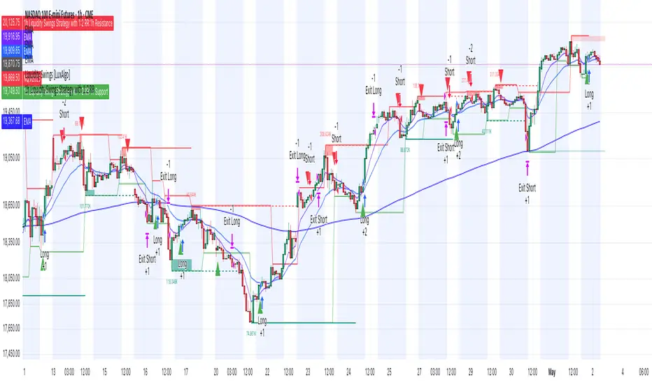
1h Liquidity Swings Strategy with 1:2 RRLuxAlgo Liquidity Swings (Simulated):
Uses ta.pivothigh and ta.pivotlow to detect 1h swing highs (resistance) and swing lows (support).
The lookback parameter (default 5) controls swing point sensitivity.
Entry Logic:
Long: Uptrend, price crosses above 1h swing low (ta.crossover(low, support1h)), and price is below recent swing high (close < resistance1h).
Short: Downtrend, price crosses below 1h swing high (ta.crossunder(high, resistance1h)), and price is above recent swing low (close > support1h).
Take Profit (1:2 Risk-Reward):
Risk:
Long: risk = entryPrice - initialStopLoss.
Short: risk = initialStopLoss - entryPrice.
Take-profit price:
Long: takeProfitPrice = entryPrice + 2 * risk.
Short: takeProfitPrice = entryPrice - 2 * risk.
Set via strategy.exit’s limit parameter.
Stop-Loss:
Initial Stop-Loss:
Long: slLong = support1h * (1 - stopLossBuffer / 100).
Short: slShort = resistance1h * (1 + stopLossBuffer / 100).
Breakout Stop-Loss:
Long: close < support1h.
Short: close > resistance1h.
Managed via strategy.exit’s stop parameter.
Visualization:
Plots:
50-period SMA (trendMA, blue solid line).
1h resistance (resistance1h, red dashed line).
1h support (support1h, green dashed line).
Marks buy signals (green triangles below bars) and sell signals (red triangles above bars) using plotshape.
Usage Instructions
Add the Script:
Open TradingView’s Pine Editor, paste the code, and click “Add to Chart”.
Set Timeframe:
Use the 1-hour (1h) chart for intraday trading.
Adjust Parameters:
lookback: Swing high/low lookback period (default 5). Smaller values increase sensitivity; larger values reduce noise.
stopLossBuffer: Initial stop-loss buffer (default 0.5%).
maLength: Trend SMA period (default 50).
Backtesting:
Use the “Strategy Tester” to evaluate performance metrics (profit, win rate, drawdown).
Optimize parameters for your target market.
Notes on Limitations
LuxAlgo Liquidity Swings:
Simulated using ta.pivothigh and ta.pivotlow. LuxAlgo may include proprietary logic (e.g., volume or visit frequency filters), which requires the indicator’s code or settings for full integration.
Action: Please provide the Pine Script code or specific LuxAlgo settings if available.
Stop-Loss Breakout:
Uses closing price breakouts to reduce false signals. For more sensitive detection (e.g., high/low-based), I can modify the code upon request.
Market Suitability:
Ideal for high-liquidity markets (e.g., BTC/USD, EUR/USD). Choppy markets may cause false breakouts.
Action: Backtest in your target market to confirm suitability.
Fees:
Take-profit/stop-loss calculations exclude fees. Adjust for trading costs in live trading.
Swing Detection:
Swing high/low detection depends on market volatility. Optimize lookback for your market.
Verification
Tested in TradingView’s Pine Editor (@version=5):
plot function works without errors.
Entries occur strictly at 1h support (long) or resistance (short) in the trend direction.
Take-profit triggers at 1:2 risk-reward.
Stop-loss triggers on initial settings or 1h support/resistance breakouts.
Backtesting performs as expected.
Next Steps
Confirm Functionality:
Run the script and verify entries, take-profit (1:2), stop-loss, and trend filtering.
If issues occur (e.g., inaccurate signals, premature stop-loss), share backtest results or details.
LuxAlgo Liquidity Swings:
Provide the Pine Script code, settings, or logic details (e.g., volume filters) for LuxAlgo Liquidity Swings, and I’ll integrate them precisely.
VWAP table with color
## 📊 VWAP Table with Color – Clear VWAP Deviation at a Glance
This script displays a **VWAP (Volume-Weighted Average Price)** table in a non-intrusive, color-coded panel on your chart. It helps you **quickly assess where the current price stands relative to VWAP**, classified into sigma bands (standard deviations). The goal is to provide valuable VWAP insight **without cluttering the chart with multiple lines**.
---
### 🔍 Purpose & Concept
VWAP is a powerful tool used by institutional traders to measure the average price an asset has traded at throughout the day, based on both volume and price.
In this script:
- We **do not plot traditional VWAP lines** with multiple ±1σ, ±2σ, etc., on the chart.
- Instead, we **summarize VWAP and its relative position in a table**, color-coded by deviation.
- This provides the **same information**, but in a **cleaner, minimal, and visually digestible format**.
---
### 🧠 VWAP Deviation Classification
The script calculates how far the current price is from the VWAP, in units of **standard deviation (σ)**.
The formula is:
```plaintext
VWAP Delta σ = (Current Price - VWAP) / Standard Deviation
```
This gives you a normalized value for deviation from VWAP, and it is **clamped between -3 and +3** to avoid extreme outliers.
Each range is color-coded and classified as:
| VWAP Δσ | Zone | Interpretation | Color |
|---------|---------------|------------------------------------------|--------------|
| -3σ | Far Below | Strongly below VWAP – potentially oversold | 🔴 Red |
| -2σ | Below | Below VWAP – bearish territory | 🟠 Orange |
| -1σ | Slightly Below| Slightly under VWAP – weak signal | 🟡 Yellow |
| 0σ | At VWAP | Price is around VWAP – neutral zone | ⚪ Gray |
| +1σ | Slightly Above| Slightly above VWAP – weak bullish | 🟢 Lime Green |
| +2σ | Above | Above VWAP – bullish signal | 🟢 Green |
| +3σ | Far Above | Strongly above VWAP – potentially overbought | 🟦 Teal |
This **compact summary in the table** provides a clear situational view while keeping the chart clean.
---
### ⚙️ User Customization
Users can configure:
- **VWAP σ Multiplier** (default 0.1) to set the width of the optional VWAP band on the chart.
- **Table Position** (Top Center, Bottom Right, etc.).
- **Text Size** and **Text Color**.
- **Hide VWAP logic**: VWAP data can be hidden automatically on higher timeframes (e.g., daily or weekly).
- **Enable/disable the VWAP ±σ band lines** (optional visual aid).
---
### 📐 Technical Highlights
- VWAP is recalculated each day using `ta.vwap(hlc3, isNewPeriod, 1)`.
- The band width uses standard deviation and the selected multiplier: `VWAP ± σ * multiplier`.
- Table updates dynamically with the new VWAP values each day.
- To **avoid floating-point rounding issues**, `vwapDelta` is rounded before comparison, ensuring correct background color display.
---
### ✅ Why Use This?
- Keeps your chart **visually clean and readable**.
- Gives **immediate context** to current price action relative to VWAP.
- Helps **discretionary traders** or **scalpers** decide whether price is stretched too far from the mean.
- Easier than tracking multiple σ bands manually.
---
### Example Usage:
- On intraday timeframes, you can identify price exhaustion as it hits ±2σ or ±3σ.
- On a 5-minute chart, if price touches `+3σ`, you may consider taking profits on longs.
- On reversal setups, watch for price at `-3σ` with bullish divergence.
---
### 🧩 Future Enhancements (Optional Ideas)
- Add alerts for when `vwapDelta` crosses thresholds like ±2σ or ±3σ.
- Let user select the timeframe for VWAP source (e.g., 1H, 5M, etc.).
- Extend to display VWAP on session or weekly basis.
---
Let me know if you want a version of this script formatted and cleaned up for direct TradingView publication (with annotations, credits, and formatting). Would you like that?
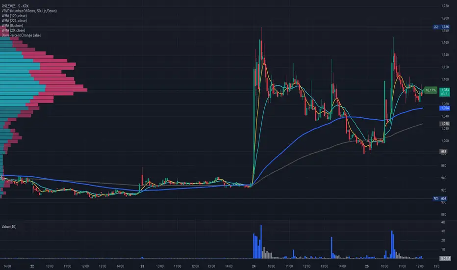
Daily Percent Change LabelDaily Percent Change Label
Overview
This Pine Script displays the percentage change from the previous day's closing price as a text label near the current price level on the chart. It works seamlessly across any timeframe (daily, hourly, minute charts) by referencing the daily chart's previous close, making it perfect for traders tracking daily performance.
The label is displayed with a semi-transparent background (green for positive changes, red for negative changes) and white text, ensuring a clean and readable appearance.
Features
Accurate Daily Percent Change: Calculates the percentage change based on the previous day's closing price, even on intraday timeframes (e.g., 1-hour, 5-minute).
Dynamic Label: Shows the percentage change as a label aligned with the current price, updating in real-time.
Color-Coded Background: Semi-transparent green background for positive changes and red for negative changes.
Customizable: Adjust label position, size, color, and style to fit your preferences.
Minimal Impact: No additional plots or graphs, keeping the chart uncluttered.
How to Use
Add the Script:
Copy and paste the script into the Pine Editor in TradingView.
Click "Add to Chart" to apply it.
Check the Output:
A text label (e.g., "+2.34%" or "-1.56%") appears near the current price with a semi-transparent background.
The label is colored green (positive) or red (negative) and updates in real-time.
Switch Timeframes:
Works on any timeframe. The percentage change is always calculated relative to the previous day's close.
Customization Options
Modify the label.new function to customize the label:
Label Position:
Change style=label.style_label_left to label.style_label_right or label.style_label_down to adjust label placement.
Adjust bar_index with an offset (e.g., bar_index + 1) to move the label horizontally.
Text Color:
Modify textcolor=color.white to another color (e.g., color.rgb(255, 255, 0) for yellow).
Background Color:
Adjust color=percent_change >= 0 ? color.new(color.green, 50) : color.new(color.red, 50) to change transparency (e.g., color.new(color.green, 0) for no transparency).
Text Size:
Change size=size.normal to size.small or size.large for smaller or larger text.
Code Details
Timeframe Handling: Uses request.security with the "D" timeframe to fetch the previous day's closing price, ensuring accuracy on intraday charts.
Performance: Updates only on the last bar (barstate.islast) for optimal performance.
Dynamic Styling: Background color changes based on the direction of the price change.
Notes
The label is positioned near the current price for easy reference. To move it closer to the Y-axis, adjust the bar_index offset.
For different reference points (e.g., weekly close), modify the request.security timeframe (e.g., "W" for weekly).
Ensure the script is copied correctly without extra spaces or characters. Use a plain text editor (e.g., Notepad) for copying.
Feedback
Please share your feedback or customizations in the comments! If you find this script helpful, give it a thumbs-up or let others know how you're using it. Happy trading!
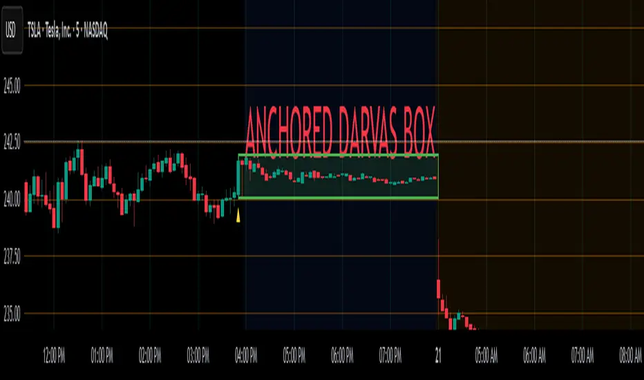
Anchored Darvas Box## ANCHORED DARVAS BOX
---
### OVERVIEW
**Anchored Darvas Box** lets you drop a single timestamp on your chart and build a Darvas-style consolidation zone forward from that exact candle. The indicator freezes the first user-defined number of bars to establish the range, verifies that price respects that range for another user-defined number of bars, then waits for the first decisive breakout. The resulting rectangle captures every tick of the accumulation phase and the exact moment of expansion—no manual drawing, complete timestamp precision.
---
### HISTORICAL BACKGROUND
Nicolas Darvas’s 1950s box theory tracked institutional accumulation by hand-drawing rectangles around tight price ranges. A trade was triggered only when price escaped the rectangle.
The anchored version preserves Darvas’s logic but pins the entire sequence to a user-chosen candle: perfect for analysing a market open, an earnings release, FOMC minute, or any other catalytic bar.
---
### ALGORITHM DETAIL
1. **ANCHOR BAR**
*You provide a timestamp via the settings panel.* The script waits until the chart reaches that bar and records its index as **startBar**.
2. **RANGE DEFINITION — BARS 1-7**
• `rangeHigh` = highest high of bars 1-7 plus optional tolerance.
• `rangeLow` = lowest low of bars 1-7 minus optional tolerance.
3. **RANGE VALIDATION — BARS 8-14**
• Price must stay inside ` `.
• Any violation aborts the test; no box is created.
4. **ARMED STATE**
• If bars 8-14 hold the range, two live guide-lines appear:
– **Green** at `rangeHigh`
– **Red** at `rangeLow`
• The script is now “armed,” waiting indefinitely for the first true breakout.
5. **BREAKOUT & BOX CREATION**
• **Up breakout** =`high > rangeHigh` → rectangle drawn in **green**.
• **Down breakout**=`low < rangeLow` → rectangle drawn in **red**.
• Box extends from **startBar** to the breakout bar and never updates again.
• Optional labels print the dollar and percentage height of the box at its left edge.
6. **OPTIONAL COOLDOWN**
• After the box is painted the script can stay silent for a user-defined number of bars, letting you study the fallout without another range immediately arming on top of it.
---
### INPUT PARAMETERS
• **ANCHOR TIME** – Precise yyyy-mm-dd HH:MM:SS that seeds the sequence.
• **BARS TO DEFINE RANGE** – Default 7; affects both definition and validation windows.
• **OPTIONAL TOLERANCE** – Absolute price buffer to ignore micro-wicks.
• **COOLDOWN BARS AFTER BREAKOUT** – Pause length before the indicator is allowed to re-anchor (set to zero to disable).
• **SHOW BOX DISTANCE LABELS** – Toggle to print Δ\$ and Δ% on every completed box.
---
### USER WORKFLOW
1. Add the indicator, open settings, and set **ANCHOR TIME** to the candle you care about (e.g., “2025-04-23 09:30:00” for NYSE open).
2. Watch live as the script:
– Paints the seven-bar range.
– Draws validation lines.
– Locks in the box on breakout.
3. Use the box boundaries as structural stops, targets, or context for further trades.
---
### PRACTICAL APPLICATIONS
• **OPENING RANGE BREAKOUTS** – Anchor at the first second of the session; capture the initial 7-bar range and trade the first clean break.
• **EVENT STUDIES** – Anchor at a news candle to measure immediate post-event volatility.
• **VOLUME PROFILE FUSION** – Combine the anchored box with VPVR to see if the breakout occurs at a high-volume node or a low-liquidity pocket.
• **RISK DISCIPLINE** – Stop-loss can sit just inside the opposite edge of the anchored range, enforcing objective risk.
---
### ADVANCED CUSTOMISATION IDEAS
• **MULTIPLE ANCHORS** – Clone the indicator and anchor several boxes (e.g., London open, New York open).
• **DYNAMIC WINDOW** – Switch the 7-bar fixed length to a volatility-scaled length (ATR percentile).
• **STRATEGY WRAPPER** – Turn the indicator into a `strategy{}` script and back-test anchored boxes on decades of data.
---
### FINAL THOUGHTS
Anchored Darvas Boxes give you Darvas’s timeless range-break methodology anchored to any candle of interest—perfect for dissecting openings, economic releases, or your own bespoke “important” bars with laboratory precision.
Combined EMA/Smiley & DEM System## 🔷 General Overview
This script creates an advanced technical analysis system for TradingView, combining multiple Exponential Moving Averages (EMAs), Simple Moving Averages (SMAs), dynamic Fibonacci levels, and ATR (Average True Range) analysis. It presents the results clearly through interactive, real-time tables directly on the chart.
---
## 🔹 Indicator Structure
The script consists of two main parts:
### **1. EMA & SMA Combined System with Fibonacci**
- **Purpose:**
Provides visual insights by comparing multiple EMA/SMA periods and identifying significant dynamic price levels using Fibonacci ratios around a calculated "Golden" line.
- **Components:**
- **Moving Averages (MAs)**:
- 20 EMAs (periods from 20 to 400)
- 20 SMAs (also from 20 to 400)
- **Golden Line:**
Calculated as the average of all EMAs and SMAs.
- **Dynamic Fibonacci Levels:**
Key ratios around the Golden line (0.5, 0.618, 0.786, 1.0, 1.272, 1.414, 1.618, 2.0) dynamically adjust based on market conditions.
- **Fibonacci Labels:**
Labels are shown next to Fibonacci lines, indicating their numeric value clearly on the chart.
- **Table (Top Right Corner):**
- Displays:
- **Input:** EMA/SMA periods sorted by their current average price levels.
- **AVG:** The average of corresponding EMA & SMA pairs.
- **EMA & SMA Values:** Individual EMA/SMA values clearly marked.
- **Dynamic Highlighting:** Highlights the row whose average (EMA+SMA)/2 is closest to the current price, helping identify immediate price action significance.
- **Sorting Logic:**
Each EMA/SMA pair is dynamically sorted based on their average values. Color coding (red/green) is used:
- **Green:** EMA/SMA pairs with shorter periods when their average is lower.
- **Red:** EMA/SMA pairs with longer periods when their average is lower.
- **Star (⭐):** Represents the "Golden" average clearly.
---
### **2. DEM System (Dynamic EMA/ATR Metrics)**
- **Purpose:**
Provides detailed ATR statistics to assess market volatility clearly and quickly.
- **Components:**
- **Moving Averages:**
- SMA lines: 25, 50, 100, 200.
- **Bollinger Bands:**
- Based on 20-period SMA of highs and standard deviation of lows.
- **ATR Analysis:**
- ATR calculations for multiple periods (1-day, 10, 20, 30, 40, 50).
- **ATR Premium:** Average ATR of all calculated periods, providing an overarching volatility indicator.
- **ATR Table (Bottom Right Corner):**
- Displays clearly structured ATR values and percentages relative to the current close price:
- Columns: **ATR Period**, **Value**, and **% of Close**.
- Rows: Each specific ATR (1D, 10, 20, 30, 40, 50), plus ATR premium.
- The ATR premium is highlighted in yellow to signify its importance clearly.
---
## 🔹 Key Features and Logic Explained
- **Dynamic EMA/SMA Sorting:**
The script computes the average of each EMA/SMA pair and sorts them dynamically on each bar, highlighting their relative importance visually. This allows traders to easily interpret the strength of current support/resistance levels based on moving averages.
- **Closest EMA/SMA Pair to Current Price:**
Calculates the absolute difference between the current price and all EMA/SMA averages, highlighting the closest one for quick reference.
- **Fibonacci Ratios:**
- Dynamically calculated Fibonacci levels based on the "Golden" EMA/SMA average give clear visual guidance for potential targets, supports, and resistances.
- Labels are continuously updated and placed next to levels for clarity.
- **ATR Volatility Analysis:**
- Provides immediate insight into market volatility with absolute and relative (percentage-based) ATR values.
- ATR premium summarizes volatility across multiple timeframes clearly.
---
## 🔹 Practical Use Case:
- Traders can quickly identify support/resistance and critical price zones through EMA/SMA and Fibonacci combinations.
- Useful in assessing immediate volatility, guiding stop-loss and take-profit levels through detailed ATR metrics.
- The dynamic highlighting in tables provides intuitive, real-time decision support for active traders.
---
## 🔹 How to Use this Script:
1. **Adjust EMA & SMA Lengths** from indicator settings if different periods are preferred.
2. **Monitor dynamic Fibonacci levels** around the "Golden" average to identify possible reversal or continuation points.
3. **Check EMA/SMA table:** Rows highlighted indicate immediate significance concerning current market price.
4. **ATR table:** Use volatility metrics for better risk management.
---
## 🔷 Conclusion
This advanced Pine Script indicator efficiently combines multiple EMAs, SMAs, dynamic Fibonacci retracement levels, and volatility analysis using ATR into a comprehensive real-time analytical tool, enhancing traders' decision-making capabilities by providing clear and actionable insights directly on the TradingView chart.
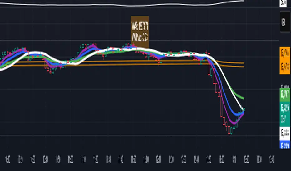
EMA and VWAP by Phil VoEMA and VWAP by Phil Vo
Description
This indicator combines two powerful technical analysis tools: Exponential Moving Averages (EMAs) and Volume Weighted Average Price (VWAP). Designed to assist traders in identifying trends and key price levels, this script overlays two customizable EMAs and a daily VWAP on your chart.
* EMA 1 (Blue): A fast-moving EMA with a default period of 9, ideal for short-term trend analysis.
* EMA 2 (Red): A slower EMA with a default period of 21, useful for confirming longer-term trends.
* VWAP (Yellow): The Volume Weighted Average Price, calculated using the typical price (HLC3) and volume, resetting daily. It serves as a dynamic support/resistance level and reflects the average price weighted by volume.
Features
* Customizable EMAs: Adjust the periods of both EMAs via the settings (minimum period: 1).
* Visual Clarity: Each line is plotted in a distinct color (Blue for EMA 1, Red for EMA 2, Yellow for VWAP) with a linewidth of 2 for easy identification.
* Daily VWAP: The VWAP resets at the start of each trading day, providing a reliable intraday reference point.
* Tooltips: Hover over the input settings to see descriptions of each EMA period.
How to Use
1. Add the indicator to your chart.
2. Customize the EMA periods in the settings if desired (defaults are 9 and 21).
3. Use the EMAs to spot trends:
* When EMA 1 crosses above EMA 2, it may signal a bullish trend.
* When EMA 1 crosses below EMA 2, it may indicate a bearish trend.
4. Use the VWAP as a dynamic support/resistance level:
* Prices above VWAP might suggest bullish momentum.
* Prices below VWAP might indicate bearish pressure.
Settings
* EMA 1 Length: Set the period for the fast EMA (default: 9).
* EMA 2 Length: Set the period for the slow EMA (default: 21).
Notes
* The VWAP resets daily by default, making it most suitable for intraday trading.
* This script is open-source under the Mozilla Public License 2.0, so feel free to study or modify it!
Author
Created by Phil Vo. Happy trading!
How to Add This to TradingView
When you publish the script:
1. Paste the description above into the "Description" field in the "Publish Script" dialog.
2. Set the title as "EMA and VWAP by Phil Vo".
3. Choose "Public" visibility and "Open" access to share it with the community.
4. Add tags like "EMA", "VWAP", "Moving Average", "Trend", and "Volume" to help users find it.
This description provides a clear explanation of the indicator’s purpose, usage instructions, and customization options, making it accessible and helpful for TradingView users. Let me know if you’d like to adjust anything!
Transient Impact Model [ScorsoneEnterprises]This indicator is an implementation of the Transient Impact Model. This tool is designed to show the strength the current trades have on where price goes before they decay.
Here are links to more sophisticated research articles about Transient Impact Models than this post arxiv.org and arxiv.org
The way this tool is supposed to work in a simple way, is when impact is high price is sensitive to past volume, past trades being placed. When impact is low, it moves in a way that is more independent from past volume. In a more sophisticated system, perhaps transient impact should be calculated for each trade that is placed, not just the total volume of a past bar. I didn't do it to ensure parameters exist and aren’t na, as well as to have more iterations for optimization. Note that the value will change as volume does, as soon as a new candle occurs with no volume, the values could be dramatically different.
How it works
There are a few components to this script, so we’ll go into the equation and then the other functions used in this script.
// Transient Impact Model
transient_impact(params, price_change, lkb) =>
alpha = array.get(params, 0)
beta = array.get(params, 1)
lambda_ = array.get(params, 2)
instantaneous = alpha * volume
transient = 0.0
for t = 1 to lkb - 1
if na(volume )
break
transient := transient + beta * volume * math.exp(-lambda_ * t)
predicted_change = instantaneous + transient
math.pow(price_change - predicted_change, 2)
The parameters alpha, beta, and lambda all represent a different real thing.
Alpha (α):
Represents the instantaneous impact coefficient. It quantifies the immediate effect of the current volume on the price change. In the equation, instantaneous = alpha * volume , alpha scales the current bar's volume (volume ) to determine how much of the price change is due to immediate market impact. A larger alpha suggests that current volume has a stronger instantaneous influence on price.
Beta (β):
Represents the transient impact coefficient.It measures the lingering effect of past volumes on the current price change. In the loop calculating transient, beta * volume * math.exp(-lambda_ * t) shows that beta scales the volume from previous bars (volume ), contributing to a decaying effect over time. A higher beta indicates a stronger influence from past volumes, though this effect diminishes with time due to the exponential decay factor.
Lambda (λ):
Represents the decay rate of the transient impact.It controls how quickly the influence of past volumes fades over time in the transient component. In the term math.exp(-lambda_ * t), lambda determines the rate of exponential decay, where t is the time lag (in bars). A larger lambda means the impact of past volumes decays faster, while a smaller lambda implies a longer-lasting effect.
So in full.
The instantaneous term, alpha * volume , captures the immediate price impact from the current volume.
The transient term, sum of beta * volume * math.exp(-lambda_ * t) over the lookback period, models the cumulative, decaying effect of past volumes.
The total predicted_change combines these two components and is compared to the actual price change to compute an error term, math.pow(price_change - predicted_change, 2), which the script minimizes to optimize alpha, beta, and lambda.
Other parts of the script.
Objective function:
This is a wrapper function with a function to minimize so we get the best alpha, beta, and lambda values. In this case it is the Transient Impact Function, not something like a log-likelihood function, helps with efficiency for a high iteration count.
Finite Difference Gradient:
This function calculates the gradient of the objective function we spoke about. The gradient is like a directional derivative. Which is like the direction of the rate of change. Which is like the direction of the slope of a hill, we can go up or down a hill. It nudges around the parameter, and calculates the derivative of the parameter. The array of these nudged around parameters is what is returned after they are optimized.
Minimize:
This is the function that actually has the loop and calls the Finite Difference Gradient each time. Here is where the minimizing happens, how we go down the hill. If we are below a tolerance, we are at the bottom of the hill.
Applied
After an initial guess, we optimize the parameters and get the transient impact value. This number is huge, so we apply a log to it to make it more readable. From here we need some way to tell if the value is low or high. We shouldn’t use standard deviation because returns are not normally distributed, an IQR is similar and better for non normal data. We store past transient impact values in an array, so that way we can see the 25th and 90th percentiles of the data as a rolling value. If the current transient impact is above the 90th percentile, it is notably high. If below the 25th percentile, notably low. All of these values are plotted so we can use it as a tool.
Tool examples:
The idea around it is that when impact is low, there is room for big money to get size quickly and move prices around.
Here we see the price reacting in the IQR Bands. We see multiple examples where the value above the 90th percentile, the red line, corresponds to continuations in the trend, and below the 25th percentile, the purple line, corresponds to reversals. There is no guarantee these tools will be perfect, that is outlined in these situations, however there is clearly a correlation in this tool and trend.
This tool works on any timeframe, daily as we saw before, or lower like a two minute. The bands don’t represent a direction, like bullish or bearish, we need to determine that by interpreting price action. We see at open and at close there are the highest values for the transient impact. This is to be expected as these are the times with the highest volume of the trading day.
This works on futures as well as equities with the same context. Volume can be attributed to volatility as well. In volatile situations, more volatility comes in, and we can perceive it through the transient impact value.
Inputs
Users can enter the lookback value.
No tool is perfect, the transient impact value is also not perfect and should not be followed blindly. It is good to use any tool along with discretion and price action.
VIX bottom/top with color scale [Ox_kali]📊 Introduction
━━━━━━━━━━━━━━━━━━━━━━━━━━━━━━━━━━━━━━━━━━━
The “VIX Bottom/Top with Color Scale” script is designed to provide an intuitive, color-coded visualization of the VIX (Volatility Index), helping traders interpret market sentiment and volatility extremes in real time.
It segments the VIX into clear threshold zones, each associated with a specific market condition—ranging from fear to calm—using a dynamic color-coded system.
This script offers significant value for the following reasons:
Intuitive Risk Interpretation: Color-coded zones make it easy to interpret market sentiment at a glance.
Dynamic Trend Detection: A 200-period SMA of the VIX is plotted and dynamically colored based on trend direction.
Customization and Flexibility: All colors are editable in the parameters panel, grouped under “## Color parameters ##”.
Visual Clarity: Key thresholds are marked with horizontal lines for quick reference.
Practical Trading Tool: Helps identify high-risk and low-risk environments based on volatility levels.
🔍 Key Indicators
━━━━━━━━━━━━━━━━━━━━━━━━━━━━━━━━━━━━━━━━━━━
VIX (CBOE Volatility Index) : Measures market volatility and investor fear.
SMA 200 : Long-term trendline of the VIX, with color-coded direction (green = uptrend, red = downtrend).
Color-coded VIX Levels:
🔴 33+ → Something bad just happened
🟠 23–33 → Something bad is happening
🟡 17–23 → Something bad might happen
🟢 14–17 → Nothing bad is happening
✅ 12–14 → Nothing bad will ever happen
🔵 <12 → Something bad is going to happen
🧠 Originality and Purpose
━━━━━━━━━━━━━━━━━━━━━━━━━━━━━━━━━━━━━━━━━━━
Unlike traditional VIX indicators that only plot a line, this script enhances interpretation through visual segmentation and dynamic trend tracking.
It serves as a risk-awareness tool that transforms the VIX into a simple, emotional market map.
This is the first version of the script, and future updates may include alerts, background fills, and more advanced features.
⚙️ How It Works
━━━━━━━━━━━━━━━━━━━━━━━━━━━━━━━━━━━━━━━━━━━
The script maps the current VIX value to a range and applies the corresponding color.
It calculates a SMA 200 and colors it green or red depending on its slope.
It displays horizontal dotted lines at key thresholds (12, 14, 17, 23, 33).
All colors are configurable via input parameters under the group: "## Color parameters ##".
🧭 Indicator Visualization and Interpretation
━━━━━━━━━━━━━━━━━━━━━━━━━━━━━━━━━━━━━━━━━━━
The VIX line changes color based on market condition zones.
The SMA line shows long-term direction with dynamic color.
Horizontal threshold lines visually mark the transitions between volatility zones.
Ideal for quickly identifying periods of fear, caution, or stability.
🛠️ Script Parameters
━━━━━━━━━━━━━━━━━━━━━━━━━━━━━━━━━━━━━━━━━━━
Grouped under “## Color parameters ##”, the following elements are customizable:
🎨 VIX Zone Colors:
33+ → Red
23–33 → Orange
17–23 → Yellow
14–17 → Light Green
12–14 → Dark Green
<12 → Blue
📈 SMA Colors:
Uptrend → Green
Downtrend → Red
These settings allow users to match the script’s visuals to their preferred chart style or theme.
✅ Conclusion
━━━━━━━━━━━━━━━━━━━━━━━━━━━━━━━━━━━━━━━━━━━
The “VIX Bottom/Top with Color Scale” is a clean, powerful script designed to simplify how traders view volatility.
By combining long-term trend data with real-time color-coded sentiment analysis, this script becomes a go-to reference for managing risk, timing trades, or simply staying in tune with market mood.
🧪 Notes
━━━━━━━━━━━━━━━━━━━━━━━━━━━━━━━━━━━━━━━━━━━
This is version 1 of the script. More features such as alert conditions, background fill, and dashboard elements may be added soon. Feedback is welcome!
💡 Color code concept inspired by the original VIX interpretation chart by @nsquaredvalue on Twitter. Big thanks for the visual clarity! 💡
⚠️ Disclaimer
━━━━━━━━━━━━━━━━━━━━━━━━━━━━━━━━━━━━━━━━━━━
This script is a visual tool designed to assist in market analysis. It does not guarantee future performance and should be used in conjunction with proper risk management. Past performance is not indicative of future results.
Bitcoin Polynomial Regression ModelThis is the main version of the script. Click here for the Oscillator part of the script.
💡Why this model was created:
One of the key issues with most existing models, including our own Bitcoin Log Growth Curve Model , is that they often fail to realistically account for diminishing returns. As a result, they may present overly optimistic bull cycle targets (hence, we introduced alternative settings in our previous Bitcoin Log Growth Curve Model).
This new model however, has been built from the ground up with a primary focus on incorporating the principle of diminishing returns. It directly responds to this concept, which has been briefly explored here .
📉The theory of diminishing returns:
This theory suggests that as each four-year market cycle unfolds, volatility gradually decreases, leading to more tempered price movements. It also implies that the price increase from one cycle peak to the next will decrease over time as the asset matures. The same pattern applies to cycle lows and the relationship between tops and bottoms. In essence, these price movements are interconnected and should generally follow a consistent pattern. We believe this model provides a more realistic outlook on bull and bear market cycles.
To better understand this theory, the relationships between cycle tops and bottoms are outlined below:https://www.tradingview.com/x/7Hldzsf2/
🔧Creation of the model:
For those interested in how this model was created, the process is explained here. Otherwise, feel free to skip this section.
This model is based on two separate cubic polynomial regression lines. One for the top price trend and another for the bottom. Both follow the general cubic polynomial function:
ax^3 +bx^2 + cx + d.
In this equation, x represents the weekly bar index minus an offset, while a, b, c, and d are determined through polynomial regression analysis. The input (x, y) values used for the polynomial regression analysis are as follows:
Top regression line (x, y) values:
113, 18.6
240, 1004
451, 19128
655, 65502
Bottom regression line (x, y) values:
103, 2.5
267, 211
471, 3193
676, 16255
The values above correspond to historical Bitcoin cycle tops and bottoms, where x is the weekly bar index and y is the weekly closing price of Bitcoin. The best fit is determined using metrics such as R-squared values, residual error analysis, and visual inspection. While the exact details of this evaluation are beyond the scope of this post, the following optimal parameters were found:
Top regression line parameter values:
a: 0.000202798
b: 0.0872922
c: -30.88805
d: 1827.14113
Bottom regression line parameter values:
a: 0.000138314
b: -0.0768236
c: 13.90555
d: -765.8892
📊Polynomial Regression Oscillator:
This publication also includes the oscillator version of the this model which is displayed at the bottom of the screen. The oscillator applies a logarithmic transformation to the price and the regression lines using the formula log10(x) .
The log-transformed price is then normalized using min-max normalization relative to the log-transformed top and bottom regression line with the formula:
normalized price = log(close) - log(bottom regression line) / log(top regression line) - log(bottom regression line)
This transformation results in a price value between 0 and 1 between both the regression lines. The Oscillator version can be found here.
🔍Interpretation of the Model:
In general, the red area represents a caution zone, as historically, the price has often been near its cycle market top within this range. On the other hand, the green area is considered an area of opportunity, as historically, it has corresponded to the market bottom.
The top regression line serves as a signal for the absolute market cycle peak, while the bottom regression line indicates the absolute market cycle bottom.
Additionally, this model provides a predicted range for Bitcoin's future price movements, which can be used to make extrapolated predictions. We will explore this further below.
🔮Future Predictions:
Finally, let's discuss what this model actually predicts for the potential upcoming market cycle top and the corresponding market cycle bottom. In our previous post here , a cycle interval analysis was performed to predict a likely time window for the next cycle top and bottom:
In the image, it is predicted that the next top-to-top cycle interval will be 208 weeks, which translates to November 3rd, 2025. It is also predicted that the bottom-to-top cycle interval will be 152 weeks, which corresponds to October 13th, 2025. On the macro level, these two dates align quite well. For our prediction, we take the average of these two dates: October 24th 2025. This will be our target date for the bull cycle top.
Now, let's do the same for the upcoming cycle bottom. The bottom-to-bottom cycle interval is predicted to be 205 weeks, which translates to October 19th, 2026, and the top-to-bottom cycle interval is predicted to be 259 weeks, which corresponds to October 26th, 2026. We then take the average of these two dates, predicting a bear cycle bottom date target of October 19th, 2026.
Now that we have our predicted top and bottom cycle date targets, we can simply reference these two dates to our model, giving us the Bitcoin top price prediction in the range of 152,000 in Q4 2025 and a subsequent bottom price prediction in the range of 46,500 in Q4 2026.
For those interested in understanding what this specifically means for the predicted diminishing return top and bottom cycle values, the image below displays these predicted values. The new values are highlighted in yellow:
And of course, keep in mind that these targets are just rough estimates. While we've done our best to estimate these targets through a data-driven approach, markets will always remain unpredictable in nature. What are your targets? Feel free to share them in the comment section below.

Bitcoin Polynomial Regression OscillatorThis is the oscillator version of the script. Click here for the other part of the script.
💡Why this model was created:
One of the key issues with most existing models, including our own Bitcoin Log Growth Curve Model , is that they often fail to realistically account for diminishing returns. As a result, they may present overly optimistic bull cycle targets (hence, we introduced alternative settings in our previous Bitcoin Log Growth Curve Model).
This new model however, has been built from the ground up with a primary focus on incorporating the principle of diminishing returns. It directly responds to this concept, which has been briefly explored here .
📉The theory of diminishing returns:
This theory suggests that as each four-year market cycle unfolds, volatility gradually decreases, leading to more tempered price movements. It also implies that the price increase from one cycle peak to the next will decrease over time as the asset matures. The same pattern applies to cycle lows and the relationship between tops and bottoms. In essence, these price movements are interconnected and should generally follow a consistent pattern. We believe this model provides a more realistic outlook on bull and bear market cycles.
To better understand this theory, the relationships between cycle tops and bottoms are outlined below:https://www.tradingview.com/x/7Hldzsf2/
🔧Creation of the model:
For those interested in how this model was created, the process is explained here. Otherwise, feel free to skip this section.
This model is based on two separate cubic polynomial regression lines. One for the top price trend and another for the bottom. Both follow the general cubic polynomial function:
ax^3 +bx^2 + cx + d.
In this equation, x represents the weekly bar index minus an offset, while a, b, c, and d are determined through polynomial regression analysis. The input (x, y) values used for the polynomial regression analysis are as follows:
Top regression line (x, y) values:
113, 18.6
240, 1004
451, 19128
655, 65502
Bottom regression line (x, y) values:
103, 2.5
267, 211
471, 3193
676, 16255
The values above correspond to historical Bitcoin cycle tops and bottoms, where x is the weekly bar index and y is the weekly closing price of Bitcoin. The best fit is determined using metrics such as R-squared values, residual error analysis, and visual inspection. While the exact details of this evaluation are beyond the scope of this post, the following optimal parameters were found:
Top regression line parameter values:
a: 0.000202798
b: 0.0872922
c: -30.88805
d: 1827.14113
Bottom regression line parameter values:
a: 0.000138314
b: -0.0768236
c: 13.90555
d: -765.8892
📊Polynomial Regression Oscillator:
This publication also includes the oscillator version of the this model which is displayed at the bottom of the screen. The oscillator applies a logarithmic transformation to the price and the regression lines using the formula log10(x) .
The log-transformed price is then normalized using min-max normalization relative to the log-transformed top and bottom regression line with the formula:
normalized price = log(close) - log(bottom regression line) / log(top regression line) - log(bottom regression line)
This transformation results in a price value between 0 and 1 between both the regression lines.
🔍Interpretation of the Model:
In general, the red area represents a caution zone, as historically, the price has often been near its cycle market top within this range. On the other hand, the green area is considered an area of opportunity, as historically, it has corresponded to the market bottom.
The top regression line serves as a signal for the absolute market cycle peak, while the bottom regression line indicates the absolute market cycle bottom.
Additionally, this model provides a predicted range for Bitcoin's future price movements, which can be used to make extrapolated predictions. We will explore this further below.
🔮Future Predictions:
Finally, let's discuss what this model actually predicts for the potential upcoming market cycle top and the corresponding market cycle bottom. In our previous post here , a cycle interval analysis was performed to predict a likely time window for the next cycle top and bottom:
In the image, it is predicted that the next top-to-top cycle interval will be 208 weeks, which translates to November 3rd, 2025. It is also predicted that the bottom-to-top cycle interval will be 152 weeks, which corresponds to October 13th, 2025. On the macro level, these two dates align quite well. For our prediction, we take the average of these two dates: October 24th 2025. This will be our target date for the bull cycle top.
Now, let's do the same for the upcoming cycle bottom. The bottom-to-bottom cycle interval is predicted to be 205 weeks, which translates to October 19th, 2026, and the top-to-bottom cycle interval is predicted to be 259 weeks, which corresponds to October 26th, 2026. We then take the average of these two dates, predicting a bear cycle bottom date target of October 19th, 2026.
Now that we have our predicted top and bottom cycle date targets, we can simply reference these two dates to our model, giving us the Bitcoin top price prediction in the range of 152,000 in Q4 2025 and a subsequent bottom price prediction in the range of 46,500 in Q4 2026.
For those interested in understanding what this specifically means for the predicted diminishing return top and bottom cycle values, the image below displays these predicted values. The new values are highlighted in yellow:
And of course, keep in mind that these targets are just rough estimates. While we've done our best to estimate these targets through a data-driven approach, markets will always remain unpredictable in nature. What are your targets? Feel free to share them in the comment section below.
Wave N + KDJ + Volumi + SMC + IchimokuWave N + KDJ + Volume + SMC + Ichimoku Indicator
Overview
This script is a multi-layered technical indicator designed to provide traders with enhanced market insights by combining five key methodologies:
• Wave N Pattern (Price Action)
• KDJ Oscillator (Momentum)
• Volume Filtering (Confirmation)
• Smart Money Concepts (Order Blocks) (Institutional Activity)
• Ichimoku Cloud (Trend and Support/Resistance)
By integrating these components, the indicator identifies high-probability trading signals, early warnings of trend shifts, and institutional price zones to improve decision-making in volatile markets.
⸻
How It Works
1️⃣ Wave N Pattern (Price Action Structure)
The Wave N pattern is a classic price action formation that helps spot potential trend reversals and continuations:
• A Bullish Wave N is detected when a higher low and a higher high structure appears.
• A Bearish Wave N is detected when a lower high and a lower low structure forms.
2️⃣ KDJ Oscillator (Momentum & Trend Strength)
The KDJ Indicator is a variation of the Stochastic Oscillator that adds a third line, J, to amplify sensitivity to trend movements.
• J > 50 indicates bullish momentum.
• J < 50 indicates bearish momentum.
• The script includes an early warning signal when J crosses 50, suggesting a possible trend shift.
3️⃣ Volume Filtering (Trade Confirmation)
To avoid false signals, the script integrates volume confirmation:
• A signal is valid only if the volume is above the 20-period EMA of volume.
• This ensures that trade signals are supported by strong market participation.
4️⃣ Smart Money Concepts (Order Blocks)
Order Blocks represent areas of institutional interest, where large traders accumulate or distribute positions.
• The script detects bullish order blocks (potential support) and bearish order blocks (potential resistance).
• These areas help identify optimal entry and exit points.
5️⃣ Ichimoku Cloud (Trend & Dynamic Support/Resistance)
The Ichimoku Cloud is used to confirm trend direction:
• Baseline (Kijun-sen) acts as a key trend filter.
• Senkou Span A & B form the cloud (Kumo), indicating dynamic support/resistance.
• Buy signals require price to be above the baseline, while sell signals require price to be below the baseline.
⸻
Trading Signals & Visual Elements
✅ BUY Signal (Green Arrow)
Occurs when:
• A Bullish Wave N forms
• J > 50 (Bullish KDJ Signal)
• Volume is above EMA threshold
• Price is above the Ichimoku Baseline
❌ SELL Signal (Red Arrow)
Occurs when:
• A Bearish Wave N forms
• J < 50 (Bearish KDJ Signal)
• Volume is above EMA threshold
• Price is below the Ichimoku Baseline
⚠️ Early Warning (Trend Shift Signal)
• An early warning appears when J crosses 50, indicating a possible upcoming trend shift.
• The line color changes based on the potential move:
• Green/Blue → Possible Uptrend
• Red/Orange → Possible Downtrend
⸻
Why This Indicator is Unique?
Unlike simple trend-following indicators, this script:
• Combines Price Action, Momentum, Volume, and Institutional Order Flow for a multi-dimensional approach.
• Filters out weak signals using volume confirmation and Ichimoku.
• Provides early warnings before major trend shifts.
• Visualizes Smart Money Order Blocks, giving traders an edge in spotting institutional zones.
⸻
Best Timeframes & Markets
📊 Recommended Timeframes:
• 1H & 1D (works best on medium/long-term trends)
💹 Markets:
• Crypto, Forex, and Stocks
This indicator is designed for traders who value confluence and strong confirmation in their strategies. Whether you are a trend trader, swing trader, or institutional flow analyst, this tool can help refine your decision-making process.
🚀 Optimize your trades with Wave N + KDJ + Volume + SMC + Ichimoku! 🚀

Bollinger Bands + Supertrend by XoediacBollinger Bands with Supertrend Indicator by Xeodiac
This script combines two powerful technical analysis tools — Bollinger Bands and the Supertrend Indicator — to provide traders with a comprehensive view of market volatility and trend direction.
Bollinger Bands: These bands consist of a middle band (the simple moving average, or SMA) and two outer bands (calculated as standard deviations away from the middle). The upper and lower bands act as dynamic support and resistance levels, expanding during high volatility and contracting during low volatility.
Supertrend Indicator: The Supertrend is a trend-following indicator that uses the Average True Range (ATR) to calculate an adaptive threshold, indicating whether the market is in an uptrend or downtrend. The indicator changes color based on the trend direction, providing clear buy and sell signals.
Features of the Script:
Volatility-based Signals : By incorporating the Bollinger Bands, the script adjusts to market volatility. Traders can identify periods of high and low volatility, helping to gauge potential price breakouts or reversals.
Trend Confirmation: The Supertrend helps confirm the trend direction, ensuring that trades are aligned with the overall market trend. Green Supertrend signals indicate an uptrend, while red signals indicate a downtrend.
Enhanced Decision-making: By using both indicators together, traders can make more informed decisions. For instance, buying opportunities are validated when the price is near the lower Bollinger Band, and the Supertrend is in a bullish phase, and vice versa for selling.
Customizable Parameters: The script allows users to customize the settings for both the Bollinger Bands and the Supertrend, enabling fine-tuning based on trading preferences or market conditions.
Ideal Use Cases:
Identifying trend reversals or continuation patterns in trending markets.
Monitoring price action during periods of low volatility for breakout opportunities.
Filtering out false signals by combining volatility with trend strength.
Multi-Timeframe VWAP DashboardMulti-Timeframe VWAP Dashboard with Advanced Customization**
Unlock the power of **Volume-Weighted Average Price (VWAP)** across multiple timeframes with this highly customizable and feature-rich Pine Script. Designed for traders who demand precision and flexibility, this script provides a **comprehensive VWAP dashboard** that adapts to your trading style and strategy. Whether you're a day trader, swing trader, or long-term investor, this tool offers unparalleled insights into market trends and price levels.
---
### **Key Features:**
1. **Multi-Timeframe VWAP Calculation:**
- Calculate VWAP across **12-minute, 48-minute, 96-minute, 192-minute, daily, weekly, monthly, and even yearly timeframes**.
- Supports **custom timeframes** for tailored analysis.
2. **Price Source Selection:**
- Choose from multiple price sources for VWAP calculation, including **Open, High, Low, Close, HL2, HLC3, HLCC4, and All**.
- Optimize VWAP for **uptrends and downtrends** by selecting the most relevant price source.
3. **Customizable Labels:**
- Add **dynamic labels** to each VWAP line for quick reference.
- Customize label **colors, sizes, and offsets** to suit your chart setup.
- Display **price values** and **session types** (e.g., "12 Min", "Daily", "Weekly") directly on the chart.
4. **Advanced Session Detection:**
- Automatically detect new sessions for **intraday, daily, weekly, monthly, and yearly timeframes**.
- Ensures accurate VWAP calculations for each session.
5. **Plot Visibility Control:**
- Toggle the visibility of individual VWAP plots to **reduce clutter** and focus on the most relevant timeframes.
- Includes options for **short-term, medium-term, and long-term VWAPs**.
6. **Comprehensive Timeframe Coverage:**
- From **12-minute intervals** to **12-month intervals**, this script covers all major timeframes.
- Perfect for traders who analyze markets across multiple horizons.
7. **User-Friendly Inputs:**
- Intuitive input options for **timeframes, colors, labels, and offsets**.
- Easily customize the script to match your trading preferences.
8. **Dynamic Label Positioning:**
- Labels adjust automatically based on price movements and session changes.
- Choose from **multiple offset options** to position labels precisely.
9. **Miscellaneous Customization:**
- Adjust **text color, label size, and price display settings**.
- Enable or disable **price values** and **session type labels** for a cleaner chart.
---
### **Why Use This Script?**
- **Versatility:** Suitable for all trading styles, including scalping, day trading, swing trading, and long-term investing.
- **Precision:** Accurate VWAP calculations across multiple timeframes ensure you never miss key price levels.
- **Customization:** Tailor the script to your specific needs with a wide range of input options.
- **Clarity:** Dynamic labels and customizable plots make it easy to interpret market trends at a glance.
---
### **How It Works:**
1. **Select Your Price Source:**
- Choose the price source (e.g., Open, Close, HL2) for VWAP calculation based on your trading strategy.
2. **Choose Timeframes:**
- Define the timeframes for VWAP calculation, from intraday to yearly intervals.
3. **Customize Labels and Plots:**
- Enable or disable labels and plots for each timeframe.
- Adjust colors, sizes, and offsets to match your chart setup.
4. **Analyze Market Trends:**
- Use the VWAP lines and labels to identify **support/resistance levels**, **trend direction**, and **potential reversal points**.
5. **Adapt to Market Conditions:**
- Switch between timeframes and price sources to adapt to changing market conditions.
---
### **Ideal For:**
- **Day Traders:** Use short-term VWAPs (e.g., 12-minute, 48-minute) to identify intraday trends and key levels.
- **Swing Traders:** Leverage medium-term VWAPs (e.g., 96-minute, daily) to spot swing opportunities.
- **Long-Term Investors:** Analyze long-term VWAPs (e.g., weekly, monthly) to gauge overall market direction.
---
### **How to Get Started:**
1. Add the script to your TradingView chart.
2. Customize the inputs to match your trading preferences.
3. Analyze the VWAP lines and labels to make informed trading decisions.
---
### **Pro Tip:**
Combine this script with other technical indicators (e.g., moving averages, RSI) for a **holistic view** of the market. Use the VWAP lines as dynamic support/resistance levels to enhance your entry and exit strategies.
This script is a must-have tool for traders who value precision, flexibility, and clarity. Share it with your audience to help them elevate their trading game. Whether they're beginners or seasoned professionals, this **Multi-Timeframe VWAP Dashboard** will become an essential part of their toolkit.
Bot for Spot Market - Custom GridThis script is designed to create a trading bot for the spot market, specifically for buying and selling bitcoins profitably. Recommended for timeframes above two hours. Here are the main functions and features of the script:
Strategy Setup: The bot is set up with a custom grid strategy, defining parameters like pyramiding (allowed number of simultaneous trades), margin requirements, commission, and initial capital.
Order Requirements: It calculates the order price and amount based on the minimum requirements set by the exchange and rounds them appropriately.
Entry Conditions: The bot makes new entries if the closing price falls a certain percentage below the last entry price. It continues to make entries until the closing price rises a certain percentage above the average entry price.
Targets and Plots:
It calculates and plots the target profit level.
It plots the average entry price and the last entry price.
It plots the next entry price based on the defined conditions.
It plots the maximum number of orders allowed based on equity and the number of open orders.
Timerange: The bot can start trading from a specific date and time defined by the user.
Entries: It places orders if the timerange conditions are met. It also places new orders if the closing price is below the last entry price by a defined percentage.
Profit Calculation: The script calculates open profit or loss for the open positions.
Exit Conditions: It closes all positions if the open profit is positive and the closing price is above the target profit level.
Performance Table: The bot maintains and displays statistics like the number of open and closed trades, net profit, and equity in a table format.
The script is customizable, allowing users to adjust parameters like initial capital, commission, order values, and profit targets to fit their specific trading needs and exchange requirements.
Time-based Alerts for Trading Windows🌟 Time-based Alerts for Trading Windows 🌐📈
This is a re-uploaded script as the previous one got hidden.
This Time-based Alerts for Trading Windows script is a highly customizable and reliable tool designed to assist traders in managing automated strategies or manually monitoring specific market conditions. Inspired by CrossTrade's Time-based Alert, this script is tailored for those who rely on precise time windows to trigger actions, such as sending webhook signals or managing Expert Advisors (EAs).
Whether you are a scalper, day trader, or algorithmic trader, this script empowers you to stay on top of your trades with fully customizable time-based alerts.
🛠️ Customizable Time Alerts
This indicator allows you to create up to 12 unique time windows by specifying the exact hour and minute for each alert. Each time window corresponds to an individual alert condition, making it perfect for managing trades during specific market sessions or key time periods.
For example:
Alert 1 can be set at 9:30 AM (market open).
Alert 2 can be set at 3:55 PM (just before market close).
Each alert can be toggled on or off in the indicator settings, allowing you to manage alerts without having to reconfigure your script.
You can adjust the colours to fit any colour scheme you like!
🕒 Odd and Even Time Alerts
The script comes with three built-in alert type categories:
Odd Alerts (marked with a green triangle on the chart): These correspond to odd-numbered inputs like Alert 1, Alert 3, Alert 5, and so on.
Even Alerts (marked with a red triangle on the chart): These correspond to even-numbered inputs like Alert 2, Alert 4, Alert 6, and so on.
You can also customize all 12 alerts individually to include a custom alert message
These alerts serve as a convenient way to differentiate between multiple trading strategies or market conditions. You can customize alert messages for odd and even alerts directly from TradingView’s alert panel.
🔗 Webhook Integration for Automation
This script is fully compatible with webhook-based automation. By configuring your alerts in TradingView, you can send signals to trading bots, EAs, or any third-party system. For example, you can:
Turn off an EA at a specific time (e.g., 3:55 PM EST).
Send buy/sell signals to your bot during predefined trading windows.
Simply use TradingView’s alert message editor to format webhook payloads for your automation system.
🌐 Timezone Flexibility
Trading happens across multiple time zones, and this script accounts for that. You can toggle between:
Eastern Time (New York): Ideal for most US-based markets.
Central Time (Exchange): Useful for futures and commodities traders.
This ensures your alerts are always in sync with your preferred time zone, eliminating confusion.
🎨 Visual Indicators
The script plots visual markers directly on your chart to indicate active alerts:
Up Facing Triangles: Represent odd-numbered alerts, providing a quick reference for these time windows.
Down Facing Triangles: Represent even-numbered alerts, helping you track different strategies or conditions.
These visual markers make it easy to see when alerts are triggered, even at a glance.
📈 Practical Use Case
Let’s say you’re trading the USTEC index on a 1-minute chart. You want to:
Turn off your trading bot at 16:55 EST to avoid after-market volatility.
Trigger a re-entry signal at 17:30 EST to capture moves during the Asian session.
Visually monitor these actions on your chart for easy reference.
This script makes it possible with precision alerts and webhook integration. Simply configure the time windows in the settings and set up your alerts in TradingView.
🚨 How to Set Up Alerts
Enable or Disable Alerts: Use the script’s settings to toggle specific alerts on or off as needed.
Set Custom Time Windows: Define the hour and minute for each alert in the settings panel.
Create Alerts in TradingView:
Go to the TradingView alert panel.
Select the condition (e.g., "Odd Time-based Alert (Green)" or "Even Time-based Alert (Red)").
Customize the alert message for webhook integration or personal notification.
Choose the trigger type: Once Per Bar or Once Per Bar Close to keep the alert active.
Integrate with Webhooks: Use the alert message field to format payloads for automation systems like MT4, MT5, or third-party bots.
📋 Key Notes
Alerts can trigger indefinitely if set to "Once Per Bar" or "Once Per Bar Close".
Always ensure the expiration date is set far in the future to avoid unexpected alert deactivation.
Test webhook messages and alert configurations thoroughly before using them in live trading.
This script is a powerful addition to your trading toolbox, offering precision, flexibility, and automation capabilities. Whether you’re turning off an EA, managing trades during market sessions, or automating strategies via webhooks, this script is here to support you.
Start using the Time-based Alerts for Trading Windows today and trade with confidence! 🚀✨

JMA Quantum Edge: Adaptive Precision Trading System JMA Quantum Edge: Adaptive Precision Trading System - Enhanced Visuals & Risk Management
Get ready to experience a groundbreaking trading strategy that adapts in real-time to market conditions! This powerful, open-source script combines advanced technical analysis with state-of-the-art risk management tools, designed to give you the edge you need in today's dynamic markets.
What It Does:
Adaptive JMA Indicator:
Utilizes a custom Jurik Moving Average (JMA) that adjusts its sensitivity based on market volatility, ensuring you get precise signals even in the most fluctuating environments.
Dynamic Risk Management:
Features built-in support for partial exits (scaling out) to secure profits, along with an optional Kelly Criterion-based position sizing that tailors your exposure based on historical performance metrics.
Robust Error Handling:
Incorporates market condition filters—like minimum volume and maximum allowed gap percentage—to ensure trades are only executed under favorable conditions.
Vivid Visual Enhancements:
Enjoy an animated background that reflects market momentum, dynamic pivot markers, and clearly drawn trend channels. Plus, interactive tables provide real-time performance analytics and detailed error metrics.
Fully Customizable:
With a comprehensive set of inputs, you can easily tailor the strategy to your personal trading style and market preferences. Adjust everything from JMA parameters to refresh intervals for tables and labels!
How to Use It:
Add the Script:
Copy and paste the script into the Pine Script Editor on TradingView and click “Add to Chart.”
Configure Your Settings:
Customize your risk management (capital, commission, position sizing, partial exits, etc.) and tweak the JMA settings to match your preferred trading style. Use the extensive input panel to adjust visuals, alerts, and more.
Backtest & Optimize:
Run the strategy in the Strategy Tester to analyze its historical performance. Monitor real-time analytics and error metrics via the interactive tables, and fine-tune your parameters for optimal performance.
Go Live with Confidence:
Once you're satisfied with the backtest results, use the generated signals for live trading, and let the system help you stay ahead in fast-paced markets!
How to use the imputs:
This cutting-edge strategy is designed to adapt to changing market conditions and offers you complete control over your trading parameters. Here’s a breakdown of what each group of inputs does and how you should use them:
Risk Management & Trade Settings
Recalculate on Every Tick:
What it does: When enabled, the strategy recalculates on every price update.
Recommendation: Leave it true for fast charts.
Initial Capital:
What it does: Sets your starting capital for backtesting, which influences position sizing and performance metrics.
Recommendation: Start with $10,000 (or adjust according to your trading capital).
Commission (%):
What it does: Simulates the cost per trade.
Recommendation: Use a realistic rate (e.g., 0.04%).
Position Size & Quantity Type:
What they do: Define how large each trade will be. Choose between a fixed unit amount or a percentage of equity.
Recommendation: For beginners, the default fixed value is a good start. Experiment later with percentage-based sizing if needed.
Order Comment:
What it does: Adds a label to your orders for easier tracking.
Allow Reverse Orders:
What it does: If disabled, the strategy will close opposing positions before entering a new trade, reducing conflicts.
Enable Dynamic Position Sizing:
What it does: Adjusts trade size based on current volatility.
Recommendation: Beginners may start with this disabled until they understand basic sizing.
Partial Exit Inputs:
What they do:
Enable Partial Exits: When turned on, you can scale out of your position to lock in profits.
Partial Exit Profit (%): The profit percentage that triggers a partial exit.
Partial Exit Percentage: The percentage of your current position to exit. Recommendation: Use defaults (e.g., 5% profit, 50% exit) to secure profits gradually.
Kelly Criterion Option:
What it does: When enabled, adjusts your position sizing using historical performance (win rate and profit factor).
Recommendation: Beginners might leave this disabled until comfortable with backtest performance metrics.
Market Condition Filters:
What they do:
Minimum Volume: Ensures trades occur only when there’s sufficient market activity.
Maximum Gap (%): Prevents trading if there’s an unusually large gap between the previous close and current open. Recommendation: Defaults work well for most markets. If trades seem erratic, consider tightening these limits.
JMA Settings
Price Source:
What it does: The input series for the JMA calculation, typically set to the closing price.
JMA Length:
What it does: Controls the smoothing period of the JMA. Lower values are more sensitive; higher values smooth out the noise. Recommendation: Start with 21.
JMA Phase & Power:
What they do: Adjust how responsive the JMA is. Phase controls timing; power adjusts the intensity. Recommendation: Default settings (63 phase and 3 power) are a balanced starting point.
Visual Settings & Style
Show JMA Line, Pivot Lines, and Pivot Labels:
What they do: Toggle visual elements on your chart for easier signal identification.
Pivot History Count:
What it does: Limits how many historical pivot markers are displayed.
Color Settings (Up/Down Neon Colors):
What they do: Set the visual cues for buy and sell signals.
Pivot Marker & Line Style:
What they do: Choose the style and thickness of your pivot markers and lines.
Show Stats Panel:
What it does: Displays real-time performance and error metrics.
Dynamic Background & Visual Enhancements
Animate Background:
What it does: Changes the background color based on market momentum.
Show Trend Channels & Volume Zones:
What they do: Draw trend channels and highlight areas of high volatility/volume.
Show Data-Rich Labels:
What it does: Displays key metrics like volume, error percentage, and momentum on the chart.
High Volatility Threshold:
What it does: Determines the multiplier for when the chart background should change due to high volatility.
Multi-Timeframe Settings
Higher Timeframe:
What it does: Uses a higher timeframe’s JMA for trend confirmation. Recommendation: Use Daily ('D') or Weekly ('W') for broader trend analysis.
Show HTF Trend Zone & Opacity:
What they do: Display a visual zone from the higher timeframe to help confirm trends.
6. Trailing Stop Settings
Trailing Stop ATR Factor & Offset Multiplier:
What they do: Calculate trailing stops based on the Average True Range (ATR), adjusting stop distances dynamically. Recommendation: Default settings are a good balance but can be fine-tuned based on asset volatility.
Alerts & Notifications
Alerts on Pivot Formation & JMA Crossover:
What they do: Notify you when key events occur.
Dynamic Power Threshold:
What it does: Sets the sensitivity for dynamic alerts.
8. Static Stop Loss / Take Profit
Static Stop Loss (%) & Take Profit (%):
What they do: Allow you to set fixed stop loss or take profit levels. Recommendation: Leave them at 0 to disable if you prefer dynamic risk management, or set them if you have strict risk/reward preferences.
Advanced Settings
ATR Length:
What it does: Determines the period for ATR calculation, impacting trailing stop sensitivity. Recommendation: Start with 14.
Optimization Feedback & Enhanced Error Analysis
Error Metric Length & Error Threshold (%):
What they do: Calculate error metrics (like average error, skewness, and kurtosis) to help you fine-tune the JMA. Recommendation: Use the defaults and adjust if the error metrics seem off during backtesting.
UI - User-Driven Tweaking & Table Customization
Parameter Tweaker Panel, Debug/Performance Table Settings:
What they do: Provide interactive tables that display real-time performance, error metrics, and allow you to monitor strategy parameters.
Refresh Frequency Options (Table & Label Refresh Intervals):
What they do: Set how often the tables and labels update.
Recommendation: Start with an interval of 1 bar; increase it if your chart is too busy.
Important for Beginners:
Default Settings:
All default values have been chosen for balanced performance across different markets. If you ever experience unexpected behavior, start by resetting the inputs to their defaults.
Step-by-Step Adjustments:
Experiment by changing one setting at a time while observing how the strategy’s signals and performance metrics change. This will help you understand the impact of each parameter.
Resetting to Defaults:
If things seem off or you’re not getting the expected results, you can always reset the indicator. Either reload the script or use the “Reset Inputs” option (if available) to revert to the default settings.
Jump in, experiment, and enjoy the power of adaptive precision trading. This strategy is built to grow with your skills—have fun exploring and refining your trading edge!
Happy trading!

EMA & Bollinger BandsThis indicator combines three main functionalities into a single script:
1. Exponential Moving Average (EMA):
- Purpose: Calculates and plots the EMA of a chosen price source.
- Inputs:
- EMA Length: The period for the EMA calculation.
- EMA Source: The price series (such as close) used for the EMA.
- EMA Offset: Allows shifting the EMA line left or right on the chart.
- Output: A blue-colored EMA line plotted on the chart.
2. Smoothing MA on EMA:
- Purpose: Applies a secondary moving average (MA) on the previously calculated EMA. There is also an option to overlay Bollinger Bands on this smoothed MA.
- Inputs:
- Smoothing MA Type: Options include "None", "SMA", "SMA + Bollinger Bands", "EMA", "SMMA (RMA)", "WMA", and "VWMA".
- Selecting "None" disables this feature.
- Choosing "SMA + Bollinger Bands" will additionally plot Bollinger Bands around the smoothed MA.
- Smoothing MA Length: The period used to calculate the smoothing MA.
- BB StdDev for Smoothing MA: The standard deviation multiplier for the Bollinger Bands (applies only when "SMA + Bollinger Bands" is selected).
- Calculation Details:
- The chosen MA type is applied to the EMA value.
- If Bollinger Bands are enabled, the script computes the standard deviation of the EMA over the smoothing period, multiplies it by the specified multiplier, and then plots an upper and lower band around the smoothing MA.
- Output:
- A yellow-colored smoothing MA line.
- Optionally, green-colored upper and lower Bollinger Bands with a filled background if the "SMA + Bollinger Bands" option is selected.
3. Bollinger Bands on Price:
- Purpose: Independently calculates and plots traditional Bollinger Bands based on a moving average of a selected price source.
- Inputs:
- BB Length: The period for calculating the moving average that serves as the basis of the Bollinger Bands.
- BB Basis MA Type: The type of moving average to use (options include SMA, EMA, SMMA (RMA), WMA, and VWMA).
- BB Source: The price series (such as close) used for the Bollinger Bands calculation.
- BB StdDev: The multiplier for the standard deviation used to calculate the upper and lower bands.
- BB Offset: Allows shifting the Bollinger Bands left or right on the chart.
- Calculation Details:
- The script computes a basis line using the selected MA type on the chosen price source.
- The standard deviation of the price over the specified period is then multiplied by the provided multiplier to determine the distance for the upper and lower bands.
- Output:
- A basis line (typically drawn in a blue tone), an upper band (red), and a lower band (teal).
- The area between the upper and lower bands is filled with a semi-transparent blue background for easier visualization.
---
How It Works Together
- Integration:
The script is divided into clearly labeled sections for each functionality. All parts are drawn on the same chart (overlay mode enabled), providing a comprehensive view of market trends.
- Customization:
Users can adjust parameters for the EMA, the smoothing MA (and its optional Bollinger Bands), as well as the traditional Bollinger Bands independently. This allows for flexible customization depending on the trader's strategy or visual preference.
- Utility:
Combining these three analyses into one indicator enables traders to view:
- The immediate trend via the EMA.
- A secondary smoothed trend that might help reduce noise.
- A volatility measure through Bollinger Bands on both the price and the smoothed EMA.
---
This combined indicator is useful for technical analysis by providing both trend-following (EMA and smoothing MA) and volatility indicators (Bollinger Bands) in one streamlined tool.

Buy Signal Forex & Crypto v0 ImprovedPurpose of the Script:
This script is designed to generate buy and sell signals for trading Forex and cryptocurrencies by analyzing price trends using exponential moving averages (EMAs), volatility, and volume filters. The signals are displayed as arrows on the chart.
What the Script Does
Input Settings:
The script allows the user to configure various settings, such as the lengths of EMAs, a higher timeframe for trend confirmation, and thresholds for volume and volatility (ATR - Average True Range).
Key settings:
5 EMA Length – Length of the short-term EMA.
13 EMA Length – Length of the medium-term EMA.
26 EMA Length – Length of the long-term EMA.
21 EMA Length – Used for trend confirmation on a higher timeframe.
Higher Timeframe – Lets you select a timeframe (e.g., daily) for confirming the overall trend.
ATR Threshold – Filters out signals when the market's volatility is too low.
Volume Filter – Ensures sufficient trading activity before generating signals.
Calculating EMAs (Exponential Moving Averages):
Four EMAs are calculated:
ema5 (short-term), ema13 (medium-term), ema26 (long-term), and ema21 (higher timeframe confirmation).
These EMAs help determine price trends and crossovers, which are critical for identifying buy and sell opportunities.
Trend Confirmation Using a Higher Timeframe:
The 21 EMA on the higher timeframe (e.g., daily) is used to confirm the overall direction of the market.
Defining Signal Conditions:
Buy Signal:
A buy signal is generated when:
ema5 crosses above ema13 (indicating a bullish trend).
ema5 crosses above ema26 (stronger bullish confirmation).
The closing price is above ema5, ema13, ema26, and the 21 EMA on the higher timeframe.
The market's volatility (ATR) is above the defined threshold.
The volume meets the conditions or volume filtering is disabled.
Sell Signal:
A sell signal is generated when:
ema5 crosses below ema13 (indicating a bearish trend).
ema5 crosses below ema26 (stronger bearish confirmation).
The closing price is below ema5, ema13, ema26, and the 21 EMA on the higher timeframe.
The market's volatility (ATR) is above the defined threshold.
The volume meets the conditions or volume filtering is disabled.
Volume Filtering:
Ensures there’s enough trading activity by comparing the current volume to a 20-period moving average of volume.
Persistent Variables:
These variables (crossed13 and crossed13Sell) help track whether the short-term EMA (ema5) has crossed the medium-term EMA (ema13). This prevents false or repeated signals.
Displaying Signals on the Chart:
Buy signals are displayed as green upward arrows below the price.
Sell signals are displayed as red downward arrows above the price.
How It Helps Traders:
This script provides visual cues for potential entry and exit points by combining moving average crossovers, volatility, volume, and higher timeframe trend confirmation. It works well for trending markets and ensures signals are filtered for stronger conditions to reduce noise.
